32 混合效应模型
\[ \def\bm#1{{\boldsymbol #1}} \]
最好找 3 个真实数据集,其中数据集 sleepstudy 和 cbpp 均来自 lme4 包。
32.1 线性混合效应模型
32.1.1 频率派
32.1.1.1 nlme
data(sleepstudy, package = "lme4")
library(nlme)
fm1 <- lme(Reaction ~ Days, random = ~ Days | Subject, data = sleepstudy)
summary(fm1)
Linear mixed-effects model fit by REML
Data: sleepstudy
AIC BIC logLik
1755.628 1774.719 -871.8141
Random effects:
Formula: ~Days | Subject
Structure: General positive-definite, Log-Cholesky parametrization
StdDev Corr
(Intercept) 24.740241 (Intr)
Days 5.922103 0.066
Residual 25.591843
Fixed effects: Reaction ~ Days
Value Std.Error DF t-value p-value
(Intercept) 251.40510 6.824516 161 36.83853 0
Days 10.46729 1.545783 161 6.77151 0
Correlation:
(Intr)
Days -0.138
Standardized Within-Group Residuals:
Min Q1 Med Q3 Max
-3.95355735 -0.46339976 0.02311783 0.46339621 5.17925089
Number of Observations: 180
Number of Groups: 18 32.1.1.2 lme4
或使用 lme4 包,可以得到同样的结果
Linear mixed model fit by REML ['lmerMod']
Formula: Reaction ~ Days + (Days | Subject)
   Data: sleepstudy

REML criterion at convergence: 1743.6

Scaled residuals:
    Min      1Q  Median      3Q     Max
-3.9536 -0.4634  0.0231  0.4634  5.1793

Random effects:
 Groups   Name        Variance Std.Dev. Corr
 Subject  (Intercept) 612.10   24.741
          Days         35.07    5.922   0.07
 Residual             654.94   25.592
Number of obs: 180, groups:  Subject, 18

Fixed effects:
            Estimate Std. Error t value
(Intercept)  251.405      6.825  36.838
Days          10.467      1.546   6.771

Correlation of Fixed Effects:
     (Intr)
Days -0.138
32.1.2 贝叶斯派
32.1.2.1 cmdstanr
32.1.2.2 brms
 Family: gaussian
  Links: mu = identity; sigma = identity
Formula: Reaction ~ Days + (Days | Subject)
   Data: sleepstudy (Number of observations: 180)
  Draws: 4 chains, each with iter = 2000; warmup = 1000; thin = 1;
         total post-warmup draws = 4000

Group-Level Effects:
~Subject (Number of levels: 18)
                    Estimate Est.Error l-95% CI u-95% CI Rhat Bulk_ESS Tail_ESS
sd(Intercept)          27.01      6.91    15.27    42.82 1.00     1655     2080
sd(Days)                6.54      1.51     4.15     9.93 1.00     1359     1917
cor(Intercept,Days)     0.08      0.30    -0.49     0.67 1.00      972     1465

Population-Level Effects:
          Estimate Est.Error l-95% CI u-95% CI Rhat Bulk_ESS Tail_ESS
Intercept   251.17      7.65   235.76   266.45 1.00     1958     2029
Days         10.37      1.72     7.01    13.81 1.00     1351     1999

Family Specific Parameters:
      Estimate Est.Error l-95% CI u-95% CI Rhat Bulk_ESS Tail_ESS
sigma    25.93      1.59    23.07    29.29 1.00     3005     2780

Draws were sampled using sampling(NUTS). For each parameter, Bulk_ESS
and Tail_ESS are effective sample size measures, and Rhat is the potential
scale reduction factor on split chains (at convergence, Rhat = 1).Computed from 4000 by 180 log-likelihood matrix
Estimate SE
elpd_loo -861.7 22.6
p_loo 34.6 8.7
looic 1723.4 45.2
------
Monte Carlo SE of elpd_loo is NA.
Pareto k diagnostic values:
Count Pct. Min. n_eff
(-Inf, 0.5] (good) 170 94.4% 592
(0.5, 0.7] (ok) 7 3.9% 571
(0.7, 1] (bad) 1 0.6% 46
(1, Inf) (very bad) 2 1.1% 7
See help('pareto-k-diagnostic') for details.
Warning message:
Found 3 observations with a pareto_k > 0.7 in model 'bm'. It is recommended to set 'moment_match = TRUE' in order to perform moment matching for problematic observations. 32.2 广义线性混合效应模型
二项分布
32.2.1 频率派
32.2.1.1 GLMMadaptive
data(cbpp, package = "lme4")
library(GLMMadaptive)
fgm1 <- mixed_model(
  fixed = cbind(incidence, size - incidence) ~ period,
  random = ~ 1 | herd, data = cbpp, family = binomial(link = "logit")
)
summary(fgm1)
Call:
mixed_model(fixed = cbind(incidence, size - incidence) ~ period,
    random = ~1 | herd, data = cbpp, family = binomial(link = "logit"))

Data Descriptives:
Number of Observations: 56
Number of Groups: 15

Model:
 family: binomial
 link: logit

Fit statistics:
   log.Lik      AIC     BIC
 -91.98337 193.9667 197.507

Random effects covariance matrix:
               StdDev
(Intercept) 0.6475934

Fixed effects:
            Estimate Std.Err z-value    p-value
(Intercept)  -1.3995  0.2335 -5.9923    < 1e-04
period2      -0.9914  0.3068 -3.2316 0.00123091
period3      -1.1278  0.3268 -3.4513 0.00055793
period4      -1.5795  0.4276 -3.6937 0.00022101

Integration:
method: adaptive Gauss-Hermite quadrature rule
quadrature points: 11

Optimization:
method: EM
converged: TRUE
32.2.1.2 lme4
或使用 lme4 包,可以得到同样的结果
fgm2 <- lme4::glmer(
  cbind(incidence, size - incidence) ~ period + (1 | herd),
  family = binomial("logit"), data = cbpp
)
summary(fgm2)
Generalized linear mixed model fit by maximum likelihood (Laplace
Approximation) [glmerMod]
Family: binomial ( logit )
Formula: cbind(incidence, size - incidence) ~ period + (1 | herd)
Data: cbpp
AIC BIC logLik deviance df.resid
194.1 204.2 -92.0 184.1 51
Scaled residuals:
Min 1Q Median 3Q Max
-2.3816 -0.7889 -0.2026 0.5142 2.8791
Random effects:
Groups Name Variance Std.Dev.
herd (Intercept) 0.4123 0.6421
Number of obs: 56, groups: herd, 15
Fixed effects:
Estimate Std. Error z value Pr(>|z|)
(Intercept) -1.3983 0.2312 -6.048 1.47e-09 ***
period2 -0.9919 0.3032 -3.272 0.001068 **
period3 -1.1282 0.3228 -3.495 0.000474 ***
period4 -1.5797 0.4220 -3.743 0.000182 ***
---
Signif. codes: 0 '***' 0.001 '**' 0.01 '*' 0.05 '.' 0.1 ' ' 1
Correlation of Fixed Effects:
(Intr) perid2 perid3
period2 -0.363
period3 -0.340 0.280
period4 -0.260 0.213 0.19832.2.1.3 mgcv
或使用 mgcv 包,可以得到近似的结果。随机效应部分可以看作可加的惩罚项
library(mgcv)
fgm3 <- gam(
  cbind(incidence, size - incidence) ~ period + s(herd, bs = "re"),
  data = cbpp, family = binomial(link = "logit"), method = "REML"
)
summary(fgm3)
Family: binomial
Link function: logit

Formula:
cbind(incidence, size - incidence) ~ period + s(herd, bs = "re")

Parametric coefficients:
            Estimate Std. Error z value Pr(>|z|)
(Intercept)  -1.3670     0.2358  -5.799 6.69e-09 ***
period2      -0.9693     0.3040  -3.189 0.001428 **
period3      -1.1045     0.3241  -3.407 0.000656 ***
period4      -1.5519     0.4251  -3.651 0.000261 ***
---
Signif. codes:  0 '***' 0.001 '**' 0.01 '*' 0.05 '.' 0.1 ' ' 1

Approximate significance of smooth terms:
         edf Ref.df Chi.sq  p-value
s(herd) 9.66     14  32.03 3.21e-05 ***
---
Signif. codes:  0 '***' 0.001 '**' 0.01 '*' 0.05 '.' 0.1 ' ' 1

R-sq.(adj) =  0.515   Deviance explained =   53%
-REML = 93.199  Scale est. = 1         n = 56
下面给出随机效应的标准差的估计及其上下限,和前面 GLMMadaptive 包和 lme4 包给出的结果也是接近的。
32.2.2 贝叶斯派
32.2.2.1 cmdstanr
32.2.2.2 brms
32.3 广义可加混合效应模型
从线性到可加,意味着从线性到非线性,可加模型容纳非线性的成分,比如高斯过程、样条。
32.3.1 频率派
32.3.1.1 mgcv (gam)
近似高斯过程、高斯过程的核函数,mgcv 包的函数 s() 帮助文档参数的说明,默认值是梅隆型相关函数及默认的范围参数,作者自己定义了一套符号约定
library(nlme)
library(mgcv)
fit_rongelap_gam <- gam(
  counts ~ s(cX, cY, bs = "gp", k = 50), offset = log(time),
  data = rongelap, family = poisson(link = "log")
)
# 模型输出
summary(fit_rongelap_gam)
Family: poisson
Link function: log

Formula:
counts ~ s(cX, cY, bs = "gp", k = 50)

Parametric coefficients:
            Estimate Std. Error z value Pr(>|z|)
(Intercept) 1.976815   0.001642    1204   <2e-16 ***
---
Signif. codes:  0 '***' 0.001 '**' 0.01 '*' 0.05 '.' 0.1 ' ' 1

Approximate significance of smooth terms:
           edf Ref.df Chi.sq p-value
s(cX,cY) 48.98     49  34030  <2e-16 ***
---
Signif. codes:  0 '***' 0.001 '**' 0.01 '*' 0.05 '.' 0.1 ' ' 1

R-sq.(adj) =  0.876   Deviance explained = 60.7%
UBRE = 153.78 Scale est. = 1 n = 157s(cX,cY)
2543.376 参数 m 接受一个向量, m[1] 取值为 1 至 5,分别代表球型 spherical, 幂指数 power exponential 和梅隆型 Matern with \(\kappa\) = 1.5, 2.5 or 3.5 等 5 种相关/核函数。
Linking to GEOS 3.11.1, GDAL 3.6.4, PROJ 9.1.1; sf_use_s2() is TRUElibrary(abind)
library(stars)
# 类型转化
rongelap_sf <- st_as_sf(rongelap, coords = c("cX", "cY"), dim = "XY")
rongelap_coastline_sf <- st_as_sf(rongelap_coastline, coords = c("cX", "cY"), dim = "XY")
rongelap_coastline_sfp <- st_cast(st_combine(st_geometry(rongelap_coastline_sf)), "POLYGON")
# 添加缓冲区
rongelap_coastline_buffer <- st_buffer(rongelap_coastline_sfp, dist = 50)
# 构造带边界约束的网格
rongelap_coastline_grid <- st_make_grid(rongelap_coastline_buffer, n = c(150, 75))
# 将 sfc 类型转化为 sf 类型
rongelap_coastline_grid <- st_as_sf(rongelap_coastline_grid)
rongelap_coastline_buffer <- st_as_sf(rongelap_coastline_buffer)
rongelap_grid <- rongelap_coastline_grid[rongelap_coastline_buffer, op = st_intersects]
# 计算网格中心点坐标
rongelap_grid_centroid <- st_centroid(rongelap_grid)
# 共计 1612 个预测点
rongelap_grid_df <- as.data.frame(st_coordinates(rongelap_grid_centroid))
colnames(rongelap_grid_df) <- c("cX", "cY")
# 预测
rongelap_grid_df$ypred <- as.vector(predict(fit_rongelap_gam, newdata = rongelap_grid_df, type = "response"))
# 整理预测数据
rongelap_grid_sf <- st_as_sf(rongelap_grid_df, coords = c("cX", "cY"), dim = "XY")
rongelap_grid_stars <- st_rasterize(rongelap_grid_sf, nx = 150, ny = 75)
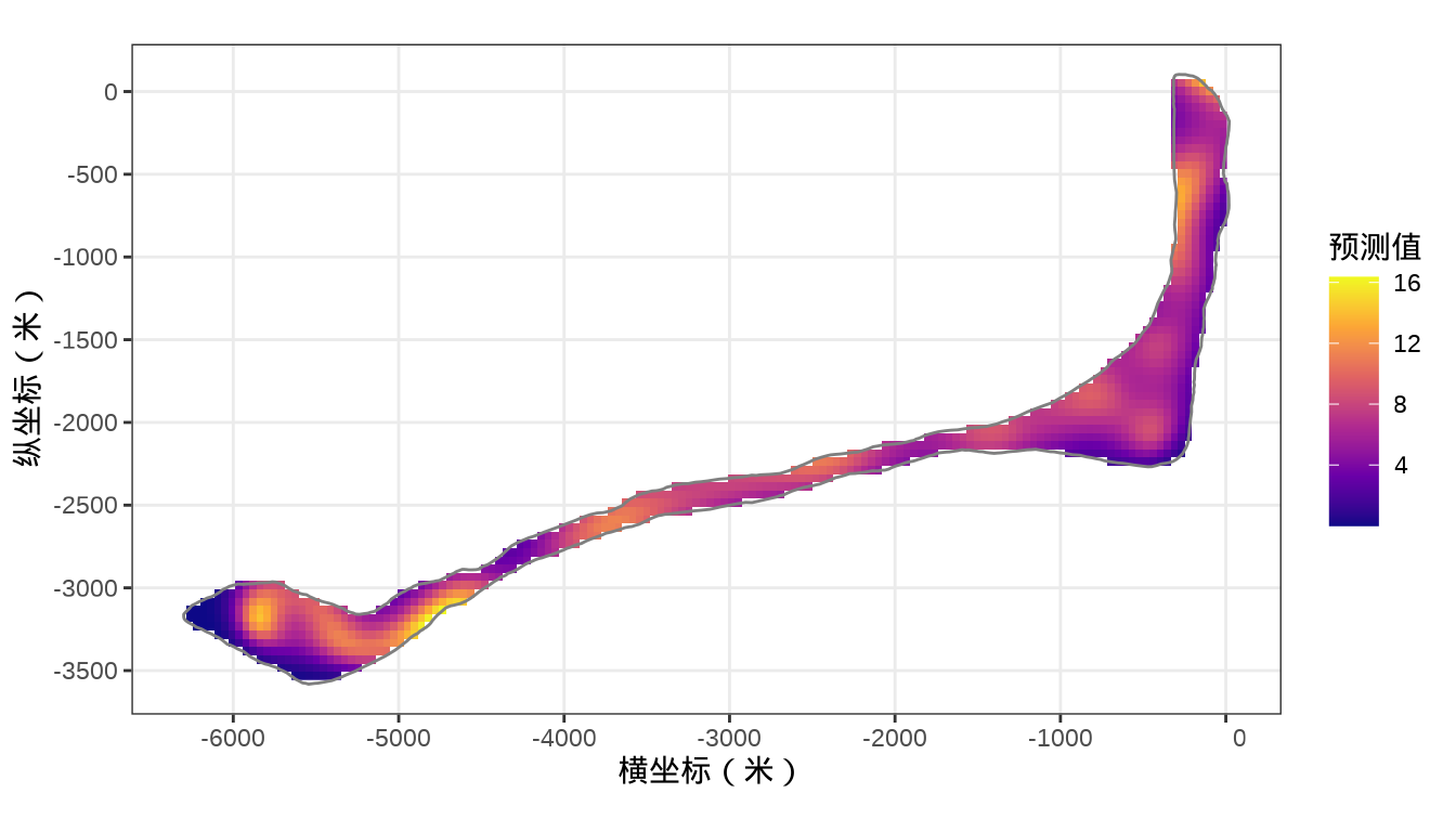
rongelap_stars <- st_crop(x = rongelap_grid_stars, y = rongelap_coastline_sfp)核辐射强度的空间分布
代码
32.3.1.2 mgcv (INLA)
mgcv 包的函数 ginla() 实现简化版 INLA
其中, \(k = 50\) 表示 50 个参数
32.3.2 贝叶斯派
32.3.2.1 brms
参考 brms 包的函数 gp() / s() 和 mgcv 包的函数 gamm() 的帮助文档,先用模拟数据检测
mgcv 包的函数 gamSim() 专门用于模拟数据。
参数 \(n=90\) 设置样本量,参数 dist = "normal" 设置变量分布,参数 eg 设置模拟数据的生成模型,取值如下
- Gu and Wahba 4 univariate term example.
- A smooth function of 2 variables.
- Example with continuous by variable.
- Example with factor by variable.
- An additive example plus a factor variable.
- Additive + random effect.
- As 1 but with correlated covariates.
'data.frame':   90 obs. of  8 variables:
 $ y  : num  3.993 -1.332 -2.834 -0.915 0.848 ...
 $ x0 : num  0.304 0.184 0.806 0.578 0.936 ...
 $ x1 : num  0.0687 0.6264 0.6771 0.1502 0.2628 ...
 $ x2 : num  0.6083 0.3385 0.0791 0.8044 0.5966 ...
 $ fac: Factor w/ 3 levels "1","2","3": 3 2 2 2 2 2 3 1 1 3 ...
 $ f1 : num  1.885 1.748 0.492 1.153 1.909 ...
 $ f2 : num  -0.383 -1.791 -2.587 1.238 -0.461 ...
 $ f3 : num  3.24 6.34 2.17 1.02 3.18 ...
模拟分组的高斯过程
32.3.2.2 INLA
INLA 近似贝叶斯计算
library(INLA)
library(splancs)
# 构造非凸的边界
boundary <- list(
  inla.nonconvex.hull(
    points = as.matrix(rongelap_coastline[,c("cX", "cY")]),
    convex = 100, concave = 150, resolution = 100),
  inla.nonconvex.hull(
    points = as.matrix(rongelap_coastline[,c("cX", "cY")]),
    convex = 200, concave = 200, resolution = 200)
)
# 构造非凸的网格
mesh <- inla.mesh.2d(
  loc = as.matrix(rongelap[, c("cX", "cY")]), offset = 100,
  max.edge = c(300, 600), boundary = boundary
)
spde <- inla.spde2.matern(mesh = mesh, alpha = 3/2, constr = TRUE)
indexs <- inla.spde.make.index(name = "s", n.spde = spde$n.spde)
lengths(indexs)

A <- inla.spde.make.A(mesh = mesh, loc = as.matrix(rongelap[, c("cX", "cY")]) )
coop <- as.matrix(rongelap_grid_df[, c("cX", "cY")])
Ap <- inla.spde.make.A(mesh = mesh, loc = coop)
dim(Ap)

# 在采样点的位置上估计 estimation stk.e
stk.e <- inla.stack(
  tag = "est",
  data = list(y = rongelap$counts, E = rongelap$time),
  A = A,
  effects = list(s = indexs)
)

# 在新生成的位置上预测 prediction stk.p
stk.p <- inla.stack(
  tag = "pred",
  data = list(y = NA, E = NA),
  A = Ap,
  effects = list(s = indexs)
)

# 合并数据 stk.full has stk.e and stk.p
stk.full <- inla.stack(stk.e, stk.p)

formula <- y ~ f(s, model = spde)

res <- inla(formula,
  data = inla.stack.data(stk.full),
  E = E, # E 已知漂移项
  control.family = list(link = "log"),
  control.predictor = list(
    compute = TRUE,
    link = 1, # 与 control.family 联系函数相同
    A = inla.stack.A(stk.full)
  ),
  control.compute = list(
    cpo = TRUE,
    waic = TRUE, # WAIC 统计量 通用信息准则
    dic = TRUE   # DIC 统计量 偏差信息准则
  ),
  family = "poisson"
)

summary(res)

res$summary.fixed
res$summary.hyperpar

index <- inla.stack.index(stk.full, tag = "pred")$data

pred_mean <- res$summary.fitted.values[index, "mean"]
pred_ll <- res$summary.fitted.values[index, "0.025quant"]
pred_ul <- res$summary.fitted.values[index, "0.975quant"]

dpm <- rbind(
  data.frame(
    cX = rongelap_grid_df[, 1], cY = rongelap_grid_df[, 2],
    value = pred_mean, variable = "pred_mean"
  ),
  data.frame(
    cX = rongelap_grid_df[, 1], cY = rongelap_grid_df[, 2],
    value = pred_ll, variable = "pred_ll"
  ),
  data.frame(
    cX = rongelap_grid_df[, 1], cY = rongelap_grid_df[, 2],
    value = pred_ul, variable = "pred_ul"
  )
)

dpm_sf <- st_as_sf(dpm, coords = c("cX", "cY"), dim = "XY")

ggplot(dpm_sf[dpm_sf$variable =="pred_mean", ]) +
  geom_sf(aes(color = value)) +
  scale_color_viridis_c(option = "C", name = expression(lambda)) +
  theme_bw()
32.4 总结
通过对频率派和贝叶斯派方法的比较,发现一些有意思的结果。
32.5 习题
-
MASS 包的地形数据集 topo 为例,高斯过程回归模型
data(topo, package = "MASS")
bgamm1 <- brms::brm(
  z ~ gp(x, y, cov = "exp_quad"),
  # family = Gamma(link = "inverse"),
  data = topo, chains = 2, seed = 20232023,
  warmup = 1000, iter = 2000, thin = 1, refresh = 0,
  control = list(adapt_delta = 0.99)
)
summary(bgamm1)
# 高斯过程近似计算
bgamm2 <- brms::brm(
  z ~ gp(x, y, cov = "exp_quad", c = 5 / 4, k = 50),
  data = topo, chains = 2, seed = 20232023,
  warmup = 1000, iter = 2000, thin = 1, refresh = 0,
  control = list(adapt_delta = 0.99)
)
summary(bgamm2)
brms 包的函数
gp()的参数 \(k\) 表示近似高斯过程 GP 所用的基函数的数目